

Welcome to the machine learning blog series. Throughout this series we'll be building and exploring machine learning technologies in the cloud and on your local machine.
In this post we will build a Iris Flower Species Classification Model using the K-Nearest Neighbors algorithm (KNN) and Python.
Let's PLAY!!
The Dataset
The Iris flower data set or Fisher’s Iris data set is a multivariate data set introduced by the British statistician and biologist Ronald Fisher in his 1936 paper. This is a very famous and widely used dataset by everyone trying to learn machine learning and statistics. The data set consists of 50 samples from each of three species of Iris (Iris setosa, Iris virginica and Iris versicolor). Four features were measured from each sample: the length and the width of the sepals and petals, in centimetres. The fifth column is the species of the flower observed.

Import Libraries
We need to import a couple of python libraries that we will need for data exploration, preprocessing, visualization and predictive modelling:
Pandas - We will be using pandas dataframes for it's functions and for a tabular representation of our dataset.
Numpy - Numerical representation of our data and calculations
Matplotlib and Seasborn - To visualize our data
ScikitLearn - To build our machine learning models.
CODE:
import pandas as pd
import numpy as np
import matplotlib.pyplot as plt
import seaborn as sns
import numpy as np
import matplotlib.pyplot as plt
import seaborn as sns
Load the Iris dataset
We will load the dataset directly from a github repository url, into a pandas dataframe.
df_Iris = pd.read_csv('https://gist.githubusercontent.com/curran/a08a1080b88344b0c8a7/raw/d546eaee765268bf2f487608c537c05e22e4b221/iris.csv')
Data Exploration
Let's take a look at the head of our dataframe (first 5 rows)
df_Iris.head()

From looking at the head of our dataset, we can identify the features and the target variable
Features include:
- sepal_length
- sepal_width
- petal_length
- petal_width
Our target label:
- species
Now let us see how many types of species there are in our dataset
df_Iris['species'].value_counts()

From looking at our output we can see that there are 3 different species as expected. And the count of each species is evenly distributed.
Let's view the shape of our dataset
df_Iris.shape

We have 150 rows and 5 columns. So that is 150 samples, 4 features and 1 target label.
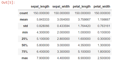
Let's view a statistical summary of our dataset
df_Iris.describe()
sns.pairplot(df_Iris, hue='species', size=3)

We can see that the setosa species is clearly distinguishable from the rest of the species, this will make it easy for our model to classify, and the rest of the species are not as easy to distinguish this will challenge the accuracy of our model.
Let's split our dataset into target and feature datasets, by assigning our feature dataset to the x variable and our target dataset to the y variable.
x = df_Iris.drop('species', axis=1)
y = df_Iris.species
Let's peek into our feature dataset
x.head()

And let's look at our target dataset
y.head()

Let's view the shape of our dataset
df_Iris.shape
We have 150 rows and 5 columns. So that is 150 samples, 4 features and 1 target label.
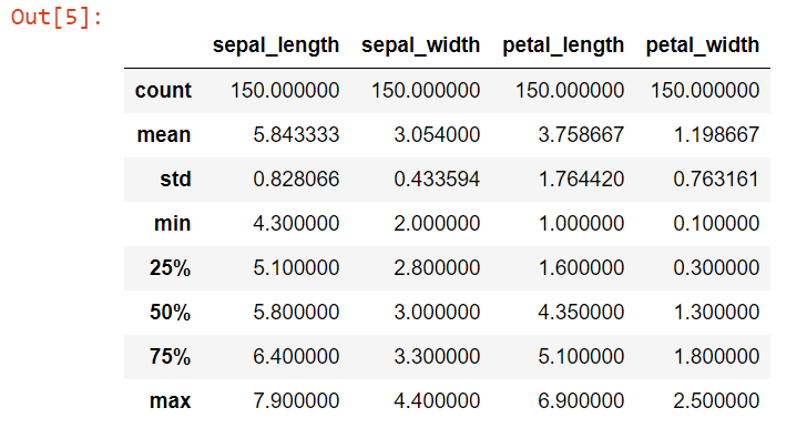
Let's view a statistical summary of our dataset
df_Iris.describe()
Data Visualization
Let's visualize our data to see if we can identify any immediate patterns. We will use seaborn to plot our data.sns.pairplot(df_Iris, hue='species', size=3)

We can see that the setosa species is clearly distinguishable from the rest of the species, this will make it easy for our model to classify, and the rest of the species are not as easy to distinguish this will challenge the accuracy of our model.
Let's split our dataset into target and feature datasets, by assigning our feature dataset to the x variable and our target dataset to the y variable.
x = df_Iris.drop('species', axis=1)
y = df_Iris.species
Let's peek into our feature dataset
x.head()

And let's look at our target dataset
y.head()

Pre-processing
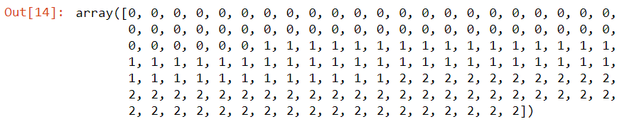
The K-Nearest Neighhors (KNN) algorithm has trouble accepting string values, so we will use Label Encoding to transform our target string values into numerical values. We will encode the Labels setosa, versicolor, and virginica into 0, 1, and 2 respectively.First let's import our label encoder from sklearn
from sklearn.preprocessing import LabelEncoder
le = LabelEncoder() # Load the label encoder
y = le.fit_transform(y) # Encode the string target features into integers
Now let's print our encoded dataset
y
Now let's split our data into testing and training datasets. We will use 70% of our dataset for training data, and 30% of our dataset for testing data.
We are going to use train_test_split from the sklearn library
from sklearn.model_selection import train_test_split
x_train, x_test, y_train, y_test = train_test_split(x, y, test_size=0.3, random_state=1)
Predictive Modelling
Let's import our KNN modelfrom sklearn.neighbors import KNeighborsClassifier
model = KNeighborsClassifier(n_neighbors=3) # Load our classifier
Now let's fit the model on our training data
model.fit(x_train, y_train)

Now let's make predictions with the trained model on our test data
prediction = model.predict(x_test)
Let's take a look at our predictions
prediction

Let's view the accuracy of our model
First we import accuracy_score from sklearn
from sklearn.metrics import accuracy_score
# Compare the accuracy of the predicted classes with the test data
accuracy = accuracy_score(y_test, prediction) * 100
Now let's print our model accuracy
print('model accuracy: ' + str(round(accuracy, 2)) + ' %.')

We have an accuracy score of 97.78 % which is pretty good.
Now let us test our model's ability to predict out of sample data
Le't s create our species dictionary so that we can use it to decode our numerical prediction value into the actual species name
# species
species = {0:'setosa',1:'versicolor',2:'virginica'}
Let's create a list of random features which the model will use to classify the type of species
x_new = [[1, 1, 1, 1]]
# make prediction
y_predict = model.predict(x_new)
Now let's see based on our new features, what type of species does the model predict
species[y_predict[0]]

Let's make another prediction
x_new = [[4, 3, 3, 2]]
y_predict = model.predict(x_new)
species[y_predict[0]]

Compare the predictions made with the pairplot graph we created above, to see if the predictions made are accurate or not. You will see the setosa species has smaller features compared to the rest and this can be seen by looking at the graph. So our first prediction we made using features [1,1,1,1] seems correct.
That marks the end of this tutorial.


